A Guide for LTE (FDD) Capacity Dimensioning
Direct to Business;
- Dont want to read calculation details, then just jump to LTEFDD-Capacity Calculator
- Feedback to aliasgherman at gmail
Introduction
(Please read this section to understand if this guide is relevant to you)
- This text is aimed to understand the LTE-FDD capacity calculations.
These are without DSS enabled.DSS based overhead calculations are also part of the document
- The text shall try to explain how a future Traffic forecast can be translated into required resources based on Statistics and Observations from current Live Network.
- Essentially, this is a practical dimensioning exercise and not a theoretical one. Difference in both approaches is that for theoretical discussion, we assume a certain overhead for all our channels and work towards building the right model, whereas for practical dimensioning we shall get all these inputs via the available Statistics and plugin to our model to get desired results.
- I shall try to divide this text into three parts.
- Theoretical background and calculations Read if you want to extend this documentation and want to gain a deeper understanding on the rationale
- Phase1 calculations which are to calculate overheads of the Control Channels only Read this for improving Control Channel Overhead knowledge
- Phase2 calculations which include Control Channel and RF condition overheads to provide final Cell Capacity This is the final product. It would require some inputs preferrably from your experience of Live network like IBLER, Rank4 ratio etc.
Theoretical Background
In simplest term, we shall work our way to list down the overall available resources for a LTE cell and then negate all the overheads we can think of. Later we shall see how to combine this with the certain efficiencies / inefficiencies introduced by the Scheduler to gain an understanding of the overall capacity.
Capacity = f_thr(AvailableRBs) - ControlOverheads - CustomizedConfigs

where,
    f_thr is a function of available RBs which provides what is the expected throughput considering all RF Conditions, Users, Resources etc.

    ControlOverheads are the overheads due to all control channels and bits like PCFICH, PSS, SSS, PBCH, DMRS, SRS etc.

    CustomizedConfigs are some additional configurations which may reduce capacity further by allocating more control resources or enabling other features such as PRS
Time Domain
| Parameter | Normal Cyclic Prefix | Extended Cyclic Prefix | Comments |
|---|---|---|---|
| Frame (ms) | 10 | 10 | Our main unit for time |
| SubFrame (ms) | 1 | 1 | |
| SubFrame in Frame (nb) | 10 | 10 | |
| Slot (ms) | 0.5 | 0.5 | 2 slots in a subframe |
| Slot in Frame (nb) | 20 | 20 | |
| Symbol per Slot (nb) | 7 | 6 | |
| Symbol per Frame (nb) | 140 | 120 | |
| Symbol (us) | 71.429 | 83.333 | 7 symbols in a slot (Normal CP), 6 symbols per slot (Extended CP) |
| Sampling Time (ns) | 32.55208333 | 32.55208333 | Sampling time considering 2048 sample size |
Frequency Domain
| Parameter | Value | Comments | Comments |
|---|---|---|---|
| Subcarriers per RB | 12 | Our main unit for time | |
| Subcarrier Spacing (KHz) | 15 | ||
| Total RB BW (KHz) | 180 | 12 subcarriers * 15KHz | 2 slots in a subframe |
RB vs. RE
A Resource Block (RB) is the smallest unit which can be allocated to a user. A Resource Element is the smallest unit representing physical layer data. Our overheads are generally calculated in terms of Resource Elements and then overall number of wasted RBs are gathered to understand overall system throughput capacity.
| Parameter | Frequency Domain (Khz) | Time Domain Symbols (Normal vs. Extended CP) | Time Domain (ms) (Normal vs. Extended) |
|---|---|---|---|
| Resource Block | 180 | 7 or 6 | 0.5 for both |
| Resource Element | 15 | 1 or 1 | 71.4us or 83.33us |
| RE in 1 RB | 12 | 7 or 6 | 1RB = 84RE (Normal CP), 72RE (Extended CP) |
Additionally, control channels are grouped together as CCEs which have the following mapping
| Item | Number of REs | Comments |
|---|---|---|
| Resource Element Group (REG) | 4 | 1 REG = 4 RE |
| Control Channel Element (CCE) | 36 | 1 CCE = 9 REG = 36 RE |
Bandwidth vs. RBs
Another table just for the sake of completeness. Below refers to the number of RBs vs. LTE total bandwidth. As you can see that the number of RBs does not cover the entire bandwidth and the rest of the frequency is mainly used as the guard band on the edge of the spectrum.
| Bandwidth | Resource Blocks |
|---|---|
| 1.4 MHz | 6 |
| 3 MHz | 15 |
| 5 MHz | 25 |
| 10 MHz | 50 |
| 15 MHz | 75 |
| 20 MHz | 100 |
Phase1 - Overhead Calculations
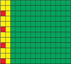
CSI-RS (Cell specific reference signals)
These symbols are the easiest to undestand as they provide the reference mathematical equations for the user. These are used by the UE to determine the RSRP and channel conditions. A specific number of REs are transmitted as CSI-RS and based on number of Antenna ports, there are certain REs on certain Antenna ports which remain as unused. The below table can be used to calculate this overhead.
| Bandwidth (Mhz) | Antenna Port | CSIRS/Subframe/RB | Total RBs | CSIRS/Frame/RB | Total CSIRS/Unused RE in Frame |
|---|---|---|---|---|---|
| 1.4 | 1 | 8 | 6 | 80 | 480 |
| 1.4 | 2 | 16 | 6 | 160 | 960 |
| 1.4 | 4 | 24 | 6 | 240 | 1440 |
| 3 | 1 | 8 | 15 | 80 | 1200 |
| 3 | 2 | 16 | 15 | 160 | 2400 |
| 3 | 4 | 24 | 15 | 240 | 3600 |
| 5 | 1 | 8 | 25 | 80 | 2000 |
| 5 | 2 | 16 | 25 | 160 | 4000 |
| 5 | 4 | 24 | 25 | 240 | 6000 |
| 10 | 1 | 8 | 50 | 80 | 4000 |
| 10 | 2 | 16 | 50 | 160 | 8000 |
| 10 | 4 | 24 | 50 | 240 | 12000 |
| 15 | 1 | 8 | 75 | 80 | 6000 |
| 15 | 2 | 16 | 75 | 160 | 12000 |
| 15 | 4 | 24 | 75 | 240 | 18000 |
| 20 | 1 | 8 | 100 | 80 | 8000 |
| 20 | 2 | 16 | 100 | 160 | 16000 |
| 20 | 4 | 24 | 100 | 240 | 24000 |
PBCH (Physical Broadcast Channel)
PBCH will use 72 subcarriers and will utilize slot1 symbol 0, 1, 2, 3. For the REs which should transmit CSI-RS in these areas, they shall not be mapped for PBCH. So, that overhead should be subtracted to not count it twice (once as CSI-RS and then as PBCH).
| Item | Frequency (subcarriers) | Time (symbols per Frame) | Total RE for PBCH | CSI-RS RE overlaps (4ports) | Only PBCH RE Overhead (per Frame) |
|---|---|---|---|---|---|
| PBCH | 72 | 4 | 288 | 48 | 240 |
PSS/SSS (Synchronization Signals)
They are the PCI carriers. Everyone knows about them, other signals want to be them. They also occupy 72 subcarriers (they use 62 and keep 10 as their buffer of unused RE) and in time domain they occur once in a half-frame. (5ms period).
| Item | Overhead RE in 1 radio Frame (includes unused unused RE on the edge) |
|---|---|
| PSS | 144 |
| SSS | 144 |
PCFICH (Physical Control Format Indicator Channel)
It uses 16 REs on symbol 0 for 1st slot of the subframe. It treats the CSI-RS space as unused but treats the CSI symbol locations as if used Antenna ports were greater than 1. So an additional overhead per frame should be considered for this case as mentioned in below table.
The additional 40 wastage should be only considered if Antenna ports =1. As PCIFCH interleaves the CSR-RS symbols as if Antenna ports used were 2 or 4 and does not use those RE positions. These then remain unused for the PCIFH symbols
| Item | Total RE/SubFrame | Total RE/Frame | Added unused RE if SISO/Frame |
|---|---|---|---|
| PCFICH | 16 | 160 | 40 |
PHICH (Physical HARQ Indicator Channel)
This is the guy which indicates ACK / NACK and is for individual user. It uses symbol 0 slot 0 for all subframes and uses subcarriers depending on the system bandwidth. There are different configuraitons for the Normal PHICH which are defined by the Number of Groups (Ng) parameter. However, even if we change this setting, the overheads will remain the same as the unused PHICH shall be transfered to PDCCH overheads in that case.
Hence, for easier mapping, below overheads for PHICH should be fine for our calculation. There is a special case where PHICH configuration can be extended which can be only used with higher CFIs for PDCCH. This seemed over-complication and so I decided to not include this in the table.
In case you are interested, with Extended PHICH, the CFI used will also be 3 for all Bandwidths, and 2 or 3 for 1.4 MHz.
Remember for 1.4MHz, Number of PDCCH symbols is CFI + 1 but for others, it is simply CFI
| Item | Bandwidth | PHICH REGs per subframe | PHICH RE per subframe | PHICH RE per Radio Frame |
|---|---|---|---|---|
| PHICH | 1.4 MHz | 3 | 12 | 120 |
| PHICH | 3 MHz | 6 | 24 | 240 |
| PHICH | 5 MHz | 12 | 48 | 480 |
| PHICH | 10 MHz | 21 | 84 | 840 |
| PHICH | 15 MHz | 30 | 120 | 1200 |
| PHICH | 20MHz | 39 | 156 | 1560 |
PDCCH (Physical Downlink Control Channel)
This is where things get interesting. The PDCCH is dynamic and varies based on cell load, selected aggregation level etc. So we have a tough choice to make while assuming the overheads of PDCCH if we want to limit our analysis on theoretical settings alone. One way of doing this can be to select the number of CFIs and then calculate the PDCCH overheads. Another way can be to get the available statistics from the Network and interpolate based on CFI usage and aggregation levels used in the sites/areas.
As we are still in the theoretical section, lets see the PDCCH REs based on CFI. Please note that the REGs and CCEs are not directly convertable as some part of REs are not sufficient to form a complete CCE and remain unused. We should consider this as a resource wastage in our calculation as well.
Overhead for 1.4/3/5MHz for CFI=1 is mentioned as zero. As per my understanding it is not possible to use CFI=1 due to insufficient Common search space CFIs. Feedback welcome for this point (aliasgherman at gmail)
| Bandwidth (MHz) | CFI | PDCCH REGs in a Frame | PDCCH CCEs in a Frame | Unuseable RE | Final PDCCH+Unused RE Overheads in Frame |
|---|---|---|---|---|---|
| 1.4 | 1 | 0 | 0 | 0 | 0 |
| 1.4 | 2 | 410 | 40 | 200 | 1640 |
| 1.4 | 3 | 590 | 60 | 200 | 2360 |
| 3 | 1 | 0 | 0 | 0 | 0 |
| 3 | 2 | 650 | 70 | 80 | 2600 |
| 3 | 3 | 1100 | 120 | 80 | 4400 |
| 5 | 1 | 0 | 0 | 0 | 0 |
| 5 | 2 | 1090 | 120 | 40 | 4360 |
| 5 | 3 | 1840 | 200 | 160 | 7360 |
| 10 | 1 | 750 | 80 | 120 | 3000 |
| 10 | 2 | 2250 | 250 | 0 | 9000 |
| 10 | 3 | 3750 | 410 | 240 | 15000 |
| 15 | 1 | 1160 | 120 | 320 | 4640 |
| 15 | 2 | 3410 | 370 | 320 | 13640 |
| 15 | 3 | 5660 | 620 | 320 | 22640 |
| 20 | 1 | 1570 | 170 | 160 | 6280 |
| 20 | 2 | 4570 | 500 | 280 | 18280 |
| 20 | 3 | 7570 | 840 | 40 | 30280 |
Dynamic Spectrum Sharing (LTE/NR)
DSS complicates the calculations. Luckily, the calculations for LTE are a bit easier to understand compared to the overheads on the NR side. DSS can be implemented via MBSFN and Non-MBSFN methods. MBSFN was introduced in LTE for eMBMS which is a method to have multi-cast data (think of it like TV broadcast). The way MBSFN works is that the cell signals the MBSFN configurations and the UE understand that for these specific subframes, the resources will be used for eMBMBS. This is useful as for the Dynamic Spectrum Sharing between LTE and NR, we can utilize these MBSFN frames as our NR signal without disturbing any non-NR legacy LTE UE.
Another possibility for DSS is to utilize Rate Matching (LTE CRS rate matching to transmit NR). MBSFN based DSS can also support a NR SCS of either 15 or 30KHz, however the non-MBSFN based DSS may only allow 30Khz SCS for NR due to limit on non-consecutive symbol availability. (Higher SCS will compress NR so it will be able to transmit 4 consecutive symbols which are required for the NR SSB. These 4 NR symbols will actually take up the sapce of 2 symbols on LTE side.)
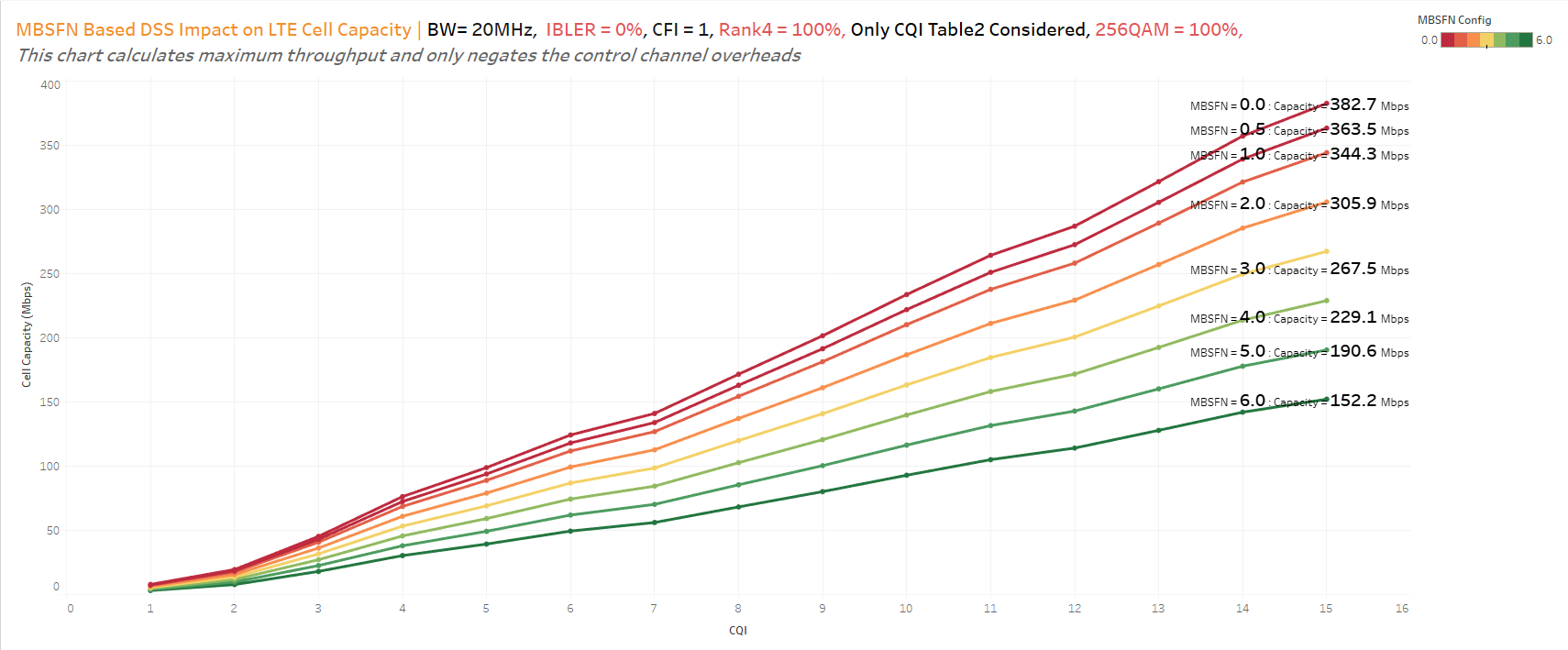
MBSFN Based DSS
During a radio frame, we may define between 0 to 6 MBSFN subframes. When a MBSFN subframe is transmitted, we still have the control channel transmissions happening on the symbols based on the CFI. As most implementations will always have variable CFIs for any subframe, this is not different as well. So we can potentially have different number of CFI symbols in a MBSFN subframe vs. others. We have already covered this point via the CFI1, CFI2, CFI3 usage ratio in our calculations.
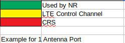
Hence, for MBSFN based DSS, our inputs are the number of MBSFN subframes in a Radio Frame only. We will then have to make sure we dont count the overheads which we have taken for all other control channels once again for these subframes.
| Number of MBSFN Subframes in a Frame | Comments | LTE Capacity Loss (%) |
|---|---|---|
| 0.5 | 1 MBSFN in 20 ms | 5 |
| 1 | 1 MBSFN in 10 ms | 10 |
| 2 | 2 MBSFN in 10 ms | 20 |
| 3 | 3 MBSFN in 10 ms | 30 |
| 4 | 4 MBSFN in 10 ms | 40 |
| 5 | 5 MBSFN in 10 ms | 50 |
| 6 | 6 MBSFN in 10 ms | 60 |
The way we can apply this scheduling loss to our calculations is as follows
(MBSFN Subframe in a Frame)/10 * (RBs * 12 * 14 * 10) - {(PHICH Overheads in Frame+ PCFICH Overheads in Frame+ PDCCH Overheads in Frame+ CRS Overheads in Frame) / 10} * (MBSFN Subframe in a Frame)
Example: for 20MHz, 4 Port Antenna, RB = 100 MBSFN Subframe in a Frame = 1 CFI1 = 100%, CFI2 = 0, CFI3 = 0, Average CFI = 1 CRS Overheads = 24000, PDCCH Overheads = 6280, PHICH Overheads = 1560, PCFICH Overheads =160 MBSFN Overheads in a frame = (1 / 10) * (100 * 12 * 14 * 10) - {(1560 + 160 + 6280 + 24000)} / 10 * (1) MBSFN Overheads in a frame = 13600 RE
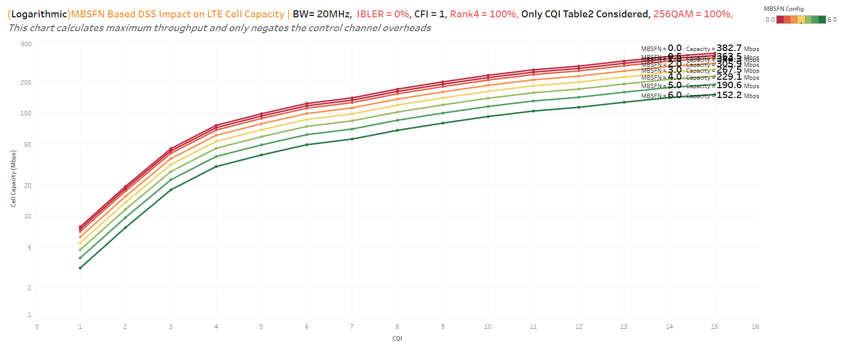
Same plot with Logarithmic capacity scale
Non-MBSFN Based DSS
These overheads will be definitely less compared to MBSFN based DSS but difficult to compute due to dynamic nature of traffic.
// TODO: Add details here
Phase 2 - PDSCH RE to Capacity
Congratulations! You made it till this part somehow. Now, we have collected the Control channel overheads and if we get all Resource Elements and subtract the Control Overheads, we would get the available REs for PDSCH. The cell capacity or throughput can be estimated based on
- Available REs for PDSCH
- CQI
- 256QAM Usage Ratio (0 - 1)
- Rank 2, 4 Usage
- IBLER
Lets briefly explore what each term means and its significance on the cell capacity.
Available RE for PDSCH
This is simplest to understand. It signifies the total available REs which we can utilize for PDSCH. Each RE can carry multiple bits of information which is based on the modulation scheme utilized. (BPSK = 1 bit, QPSK = 2, 16QAM = 4, 64QAM = 6, 256QAM = 8). The factor of used Modulation Schemes will come into our calculations with the usage of CQI to MCS tables and 256QAM usage percentage.
256QAM Ratio
This value from 0 - 1 will indicate how much traffic uses 256QAM modulation scheme. 3GPP 36.213 specifies two CQI to MCS tables alongwith the Code Rate (amount of information bits + amount of redundant bits) / (transport block size in bits). The first table is utilized when reported CQI mapping is for scenarios without 256QAM usage and the second table is when 256QAM is used. For our calculations, we use these tables like below
calculated_efficiency = 64qam_efficiency_table_for_cqi_X * (1 - 256QAM_Ratio) + 256qam_efficiency_table_for_cqi_X * (256QAM_Ratio) Where, 64qam_efficiency_table_for_cqi_X is the interpolated value of efficiency from 3gpp Table 7.2.3-1 for CQI = X 256qam_efficiency_table_for_cqi_X is the interpolated value of efficiency from 3gpp Table 7.2.3-2 for CQI = X
Rank2 , 4 Ratio
As we calculated the overheads in control channels, we noticed that with higher Antenna ports, the overheads are different. Theoretically, with perfect orthogonality for users receiving streams from all antennas, we can transmit completely different streams on each antenna port. This essentially means that with 4 port antenna, we can potentitally have 4 times the data rate. This is where the Rank 2-4 % comes in useful. If we utilize the KPIs or design values for the Rank 2 ratio, we would consider this amount of PDSCH available RE to be able to provide double the throughput. So, it is important to not consider all 4 ports as potentially 4 times the cell capacity as this depends heavily on RF conditions and UE capabilities. Indeed, it is a better idea to incorporate the Rank indications to get to a more realistic picture of how much capacity an actual MIMO system will provide over a SISO configuration.
IBLER
Well, MAC layer is tough. Just like life. Not all packets are decoded the first time. The scheduler is designed to balance between allocated MCS and RBs in a way to converge to a configured initial block error rate (IBLER). This means that the PDSCH resources will be used to retransmit this amount of data bits so it should not be counted as a useable throughput during capacity calculations.
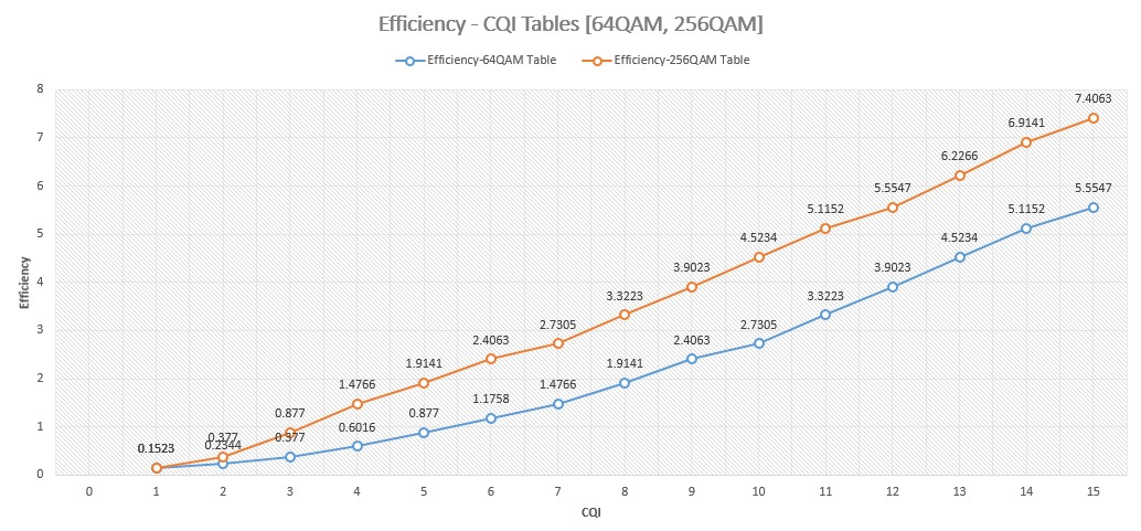
CQI to MCS Tables
Lets first put down the CQI-MCS tables below.
Table 1 - 64QAM
| CQI index | modulation | code rate x 1024 | efficiency |
|---|---|---|---|
| 0 | out of range | ||
| 1 | QPSK | 78 | 0.1523 |
| 2 | QPSK | 120 | 0.2344 |
| 3 | QPSK | 193 | 0.377 |
| 4 | QPSK | 308 | 0.6016 |
| 5 | QPSK | 449 | 0.877 |
| 6 | QPSK | 602 | 1.1758 |
| 7 | 16QAM | 378 | 1.4766 |
| 8 | 16QAM | 490 | 1.9141 |
| 9 | 16QAM | 616 | 2.4063 |
| 10 | 64QAM | 466 | 2.7305 |
| 11 | 64QAM | 567 | 3.3223 |
| 12 | 64QAM | 666 | 3.9023 |
| 13 | 64QAM | 772 | 4.5234 |
| 14 | 64QAM | 873 | 5.1152 |
| 15 | 64QAM | 948 | 5.5547 |
Table 1 - 256QAM
| CQI index | modulation | code rate x 1024 | efficiency |
|---|---|---|---|
| 0 | out of range | ||
| 1 | QPSK | 78 | 0.1523 |
| 2 | QPSK | 193 | 0.377 |
| 3 | QPSK | 449 | 0.877 |
| 4 | 16QAM | 378 | 1.4766 |
| 5 | 16QAM | 490 | 1.9141 |
| 6 | 16QAM | 616 | 2.4063 |
| 7 | 64QAM | 466 | 2.7305 |
| 8 | 64QAM | 567 | 3.3223 |
| 9 | 64QAM | 666 | 3.9023 |
| 10 | 64QAM | 772 | 4.5234 |
| 11 | 64QAM | 873 | 5.1152 |
| 12 | 256QAM | 711 | 5.5547 |
| 13 | 256QAM | 797 | 6.2266 |
| 14 | 256QAM | 885 | 6.9141 |
| 15 | 256QAM | 948 | 7.4063 |
If we explore these tables, we will see that efficiency is almost a linear function of CQI for both tables. Indeed, 256QAM pushes the efficiency higher quicker compared to 64QAM. The tradeoff is that with such implementations, if a scheduler pushes for 256QAM more and more, the block error rates will also increase due to the increased interference (256QAM will have higher power requirements due to 256 I/Q combinations and without higher power these will be extremely close to each other causing decoding errors).
Phase 2 - Calculations
Assume,
    Remaining RE for PDSCH (WITHOUT CONSIDERING MIMO GAIN) = n_re_pdsch_wo_mimo
    IBLER_Ratio = 0.12 //12% Initial block error rate
    CQI = 10.3 //Average CQI values in cell
    Rank2_Ratio = 0.45 //45% Rank2 PRB Usage.
    Rank3_Ratio = 0.05 //
    Rank4_Ratio = 0.02 //2% Rank4 PRB Usage.
    256QAM_Usage = 0.09 //9% 256QAM Usage in the cell

Then,
    We need to first interpolate the CQI to MCS table for non integer values. This means we have to calculate the Efficiency Factor for both Table1 and Table 2 for a CQI value of 10.3 (as given in our input parameters above).

    Table1
    CQI = 10 Efficiency_EF1: 2.7305, CQI = 11 Efficiency_EF2: 3.3223
    For CQI = 10.3,
        Efficiency = (Efficiency_EF2 - Efficiency_EF1) * (10.3 - 10) + Efficiency_EF1

    The above formula is simply considering the slope of line formula (y = mx + b), and trying to add the efficiency of CQI=10 and then adding the efficiency based on the slope between efficiency of CQI 11 and CQI 10.

    n_efficiency = Efficiency_table1 * (1 - 256QAM_Usage) + Efficiency_table2 * (256QAM_Usage)
Considering that you did read the above paragraph, the final Cell Capacity would be calculated as,
Cell Capacity (Mbps) = (100) * n_re_pdsch_wo_mimo x n_efficiency x (1 * (1 - Rank2_Ratio - Rank3_Ratio - Rank4_Ratio) + 2 * Rank2_Ratio + 3 * Rank3_Ratio + 4 * Rank4_Ratio) x (1 - IBLER_Ratio) / 1024 / 1024

* 100 multiplication is there because we calculated PDSCH RE for 1 frame. There are 100 frames in a second. (1000 TTIs).
(1 * (1 - Rank2_Ratio - Rank3_Ratio - Rank4_Ratio) + 2 * Rank2_Ratio + 3 * Rank3_Ratio + 4 * Rank4_Ratio) : This term is trying to calculate the usage of Rank1 and others and then multiplies the gain with the capacity considering that Rank2 essentially means double the capacity and so on.
Phew. This was too much indeed. You have now earned the right to go to the LTEFDD-Capacity Calculator and perform capacity calculations.